Analysing steepness induced fatigue in road-cyclists
A self-analysis of GPS data in R
Code
library("readr")
library("sf")
library("ggplot2")
library("dplyr")
library("tmap")
library("terra")
library("ggspatial")
library("cowplot")
Abstract
When a cyclist rides up a hill, they tend to get more tired. Or do they? In this project the author tries to analyse his own data to find out if there is a noticeable and statistically significant effect of steep hills on his riding speed. From his own experience, he does tend to slow down after a hill, but recovers rather quickly. This project tries to lay a framework for using GPS (Global Positioning System) data and Digital Elevation model (DEM) height data to answer this question. The project manages to create a framework in R, but it could not answer the question conclusively.
Introduction
When cycling in Switzerland, hills are omnipresent and going up- or downhill is nearly inevitable. Cyclists therefore go up and down which influences their efficiency, with steep gradients of more than 10-15% being less efficient than walking (Ardigò, Seibene, and Minetti 2003). The author of this paper was interested whether cyclists slow down after a steep hill and whether they speed up again after a while. This seemed logical to the author, mainly due to his own experiences.
This led to the following Research Question and Hypotheses:
RQ: Do cyclists slow down after a steep segment of their route compared to just
before the steep segment?
H1: They tend to get slower after a steep segment.
H2: They recover after a while to the level before the steep segment, but
eventually there is a fatigue effect over one journey.
H3: There is a training effect over multiple journeys.
To explore this Research Question, a movement analysis was performed in R. According to a preliminary literature review, there has not been much research on the topic of steep gradients for cyclists in the GIS field. Parkin and Rotheram (2010) refer to steep gradients for cyclists starting from 3% slope, where the cyclists mean speed starts to fall off and the slope is ‘being felt’. Castro, Johansson, and Olstam (2022) expanded on Parkin and Rotheram (2010) idea, but they were more interested in acceleration over the gradient than in the speed after the gradient. Their simulation results show that some cyclists have enough power to maintain their speed over long uphill stretches, but they also note that this would not be expected in real-life scenarios. Winters et al. (2016) used a gradient in their cycling score calculations, but only considered 2-10% as differentiated gradients. It is not stated whether this was due to the study area or other factors, but it means that more than 10% is deemed as hard as it gets. Similarly, Cho et al. (1999) describe a slope of 0-15% in their study on gear ratios, but do not elaborate why they chose that range, implying that above 15% there is not much difference for their system. Even considering papers from Kinesiology and Physiology ((Duc et al. 2008); (Swinnen, Laughlin, and Hoogkamer 2022)) there seems to not be a consent on what is considered steep. Aggregating this all together, there seems to not be a consent on what is steep and most authors design their own parameters as they see fit. For this study, this means that the approach is mostly free form and designed by the author. The starting point of a 3% gradient was chosen in this paper. The algorithm that was used to segment the data and to calculate speed was modified from (Laube and Purves 2011) and based on Algorithms taught in the UZH course: GEO880 Computational Movement Analysis.
Material and Methods
Data
GPS data
The data used for this analysis is cycling data recorded with the movement tracking app POSMO over multiple trips by the author in Switzerland between Würenlos and Altstetten (Figure 1). The GPS data is recorded every 10 seconds and the data collection was done on 8 days between April 7th and Mai 21st. The data has been pre-processed, so that only longer (around an hour or more) cycling trips are included. The data is verified, meaning that the GPS location is rather precise and no outliers were found visually. The data was also cropped, so that the home location cannot be exactly determined. This resulted in 2126 data points (overview in Table 1).
Code
# Reading in Posmo Data, cropping it so that home location is not shown and filter bike data
posmo <- read_delim("datasets/posmo_2023-04-07T00_00_00+02_00-2023-06-02T23_59_59+02_00.csv")

# make sure lat and long do not have na values
posmo<-posmo[!is.na(posmo$lon_x),]
posmo<-posmo[!is.na(posmo$lat_y),]

posmo_sf <- st_as_sf(posmo, coords = c("lon_x", "lat_y"), crs = 4326, remove = FALSE)

posmo_sf <- st_transform(posmo_sf, crs = 2056)

# filter out home coordinates
# make polygon https://www.keene.edu/campus/maps/tool/
p1 = st_point(c(8.4265439, 47.3955710))
p2 = st_point(c(8.4267632, 47.3898521))
p3 = st_point(c(8.4179950, 47.3890680))
p4 = st_point(c(8.4178061, 47.3923967))

# make polygon
poly = st_multipoint(c(p1, p2, p3, p4)) %>%
  st_cast("POLYGON") %>%
  st_sfc(crs = 4326) %>%
  st_transform(crs = 2056)

# create function that 'cuts' out the area covered by the polygon
not_covered_by  = function(x, y) !st_covered_by(x, y)

#leave out everything that's not bike data, filter the polygon, also leave out 4-11-2023, 4-25-2023 and 4-28-2023, because that was not a bike tour, only very short trips
posmo_sf_cut <- posmo_sf |>
  filter(transport_mode == "Bike")%>%
  st_filter(poly, .predicate=not_covered_by) |>
  ungroup() |>
  mutate(
    datetime = as.POSIXct(datetime),
    date = lubridate::date(datetime)
    ) |>
  filter(date != as.Date('2023-04-11') & date != as.Date('2023-04-25') & date != as.Date('2023-04-28')) |>
  select(-user_id, -place_name)

tmap_mode("view")
tm_shape(posmo_sf_cut) +
tm_dots("date") Code
knitr::kable(head(posmo_sf_cut, n= 3))| datetime | weekday | transport_mode | lon_x | lat_y | geometry | date |
|---|---|---|---|---|---|---|
| 2023-04-07 15:32:10 | Fri | Bike | 8.417895 | 47.39294 | POINT (2673932 1249584) | 2023-04-07 |
| 2023-04-07 15:32:20 | Fri | Bike | 8.417842 | 47.39350 | POINT (2673928 1249648) | 2023-04-07 |
| 2023-04-07 15:32:30 | Fri | Bike | 8.417596 | 47.39382 | POINT (2673909 1249682) | 2023-04-07 |
DEM
To calculate the slope, a Digital Elevation Model (DEM) of Switzerland with a 0.5 meter resolution from swissALTI3D (Federal Office of Topography swisstopo 2021) was used. The relevant tiles were hand-picked (Figure 2) to cover roughly the same extent as the cycling data . This resulted in 190 tiles of 1km x 1km.

Methods
Height
To use the elevation together with the cycling data, they had to be joined. Loading all DEM raster tiles into memory was not feasible and would have taken a lot of time. With the R package terra, this was made easy, as it only loads references into memory that are actually used. A virtual raster layer was created, which references all tiles, which then was loaded as a raster layer that was then made plottable (see Figure 3). This method does not allow for more nuanced plotting with packages like ggplot, as they require the data to be in memory.
The DEM height attribute was then extracted and added to the cycling data points as can be seen in Figure 4, drawn with the R package Tmap (Tennekes 2018).
Code
#csv has all download paths from alti3d tiles  https://www.swisstopo.admin.ch/en/geodata/height/alti3d.html
all_tif <- read.csv("datasets/alti3D_all.csv", header = FALSE)

# terra help https://rspatial.org/spatial-terra/8-rastermanip.html

#download all files to folder, commented out because it only has to run once
# for (fi in all_tif$V1){
#   outfile <- basename(fi)
#
#   print(outfile)
#
#   download.file(fi, paste0("datasets/alti3d_05/", outfile),mode = "wb")  # mode (binary) very important
# }

# takes all files with .tif from a folder
file_list <- list.files("datasets/alti3d_05",".tif",full.names = TRUE)

# makes a virtual raster layer from the files
vrt(file_list, "altivrt.vrt",overwrite = TRUE)

# import the data from the virtual raster layer
virt_rast <- rast("altivrt.vrt")

plot(virt_rast)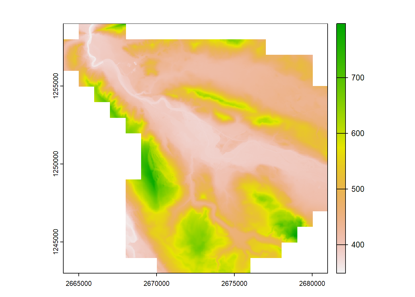
Code
DEM <- extract(virt_rast, posmo_sf_cut)

posmo_sf_cut$height <- DEM$altivrt

tm_shape(posmo_sf_cut) +
tm_dots("height") Speed and Stops
The following approach was adopted from Laube and Purves (2011). To calculate the speed, a temporal window of 1 was used, this means that the distance for each point was calculated to the one before and after. This distance was then divided by the time difference of these points and multiplied by 3.6 to get kilometers per hour. The data was then filtered for points that represent stops in movement (like breaks). Laube and Purves (2011) did this by comparing average distances within the moving window. For this study, the stopping criterion was adapted such that a cyclist is considered stopped when the average speed of the current, the previous and next point is less than 1 km/h, or if the distance covered from the last point or to the next point is less than 2 meters. This criterion was empirically tested on the data. The points that were determined to be stops where then excluded from the data which resulted in Figure 5.
Code
# temporal window, need N and E, take that from geometry column, add a grouping column date, use lead and lag to compute euclidian distances (which works thanks to Swiss Coordinate system)
bike <- posmo_sf_cut |>
  mutate(E = st_coordinates(geometry)[,1]) |>
  mutate(N = st_coordinates(geometry)[,2]) |>
  group_by(date) |>
    mutate(
        nMinus1 = sqrt((lag(N, 1) - N)^2 + (lag(E, 1) - E)^2), # distance to pos -10 sec
        nPlus1  = sqrt((N - lead(N, 1))^2 + (E - lead(E, 1))^2), # distance to pos +10 sec
    ) |>
  ungroup()

# speed, defined as the average of step behind and step in front divided by the timedifference of datetime of these two steps. *3.6 to get km/h
bike <- bike |>
  mutate(
    speed = ((nPlus1 + nMinus1)/as.integer(difftime(lead(datetime), lag(datetime), "secs")))*3.6
  )

bike <- bike |>
    ungroup() |>
    mutate(static = ifelse((speed + lead(speed) + lag(speed))/3 < 1, TRUE, nPlus1 < 2 | nMinus1 < 2))

# bike |>
#   ggplot(aes(E, N)) +
#   geom_path() +
#   geom_point(aes(color = static), alpha = 0.3) +
#   coord_fixed()

bike_filter <- bike |>
    filter(!static)

tm_shape(bike_filter) +
tm_dots("speed") Gradient
To calculate the gradient of each point, the distance to the next point was divided by the height difference to that point and multiplied by 100 to get percent (Figure 6), as is standard for road gradients. There were some end points of routes that calculated to 400% gradient. Therefore a filter was set to exclude points with more than +-50% gradient. Then, the decision to smooth the gradient with a moving window (+-1 point) was made, so that there are no extreme jumps (before the smoothing, the max gradient was +40% and min gradient was -30%, which is unlikely in this study area).
This led to the distribution presented on the right in Figure 7, which looks normally distributed with not many outliers, opposed to the figure on the left in Figure 7. This would be expected for continuous cycling data. The gradient added to the data points can be seen in Figure 8.
Code
bike_gradient <- bike_filter |>
  mutate(
    gradient = (lead(height)-height)/nPlus1*100
  )

hist1 <- ggplot(bike_gradient, aes(gradient)) +
  geom_histogram(binwidth = 1)

bike_gradient <- bike_gradient |>
  filter(gradient < 50 ) |>
  filter(gradient > -50) |>
  mutate(
    gradientplus1 = lead(gradient),
    gradientminus1 = lag(gradient)
  ) |>
  rowwise() |>
  mutate(
    gradient_smooth = mean(c(gradient, gradientplus1, gradientminus1))
    ) |>
  ungroup()

hist2 <- ggplot(bike_gradient, aes(gradient_smooth)) +
  geom_histogram(binwidth = 1)

plot_grid(hist1, hist2, cols = 2)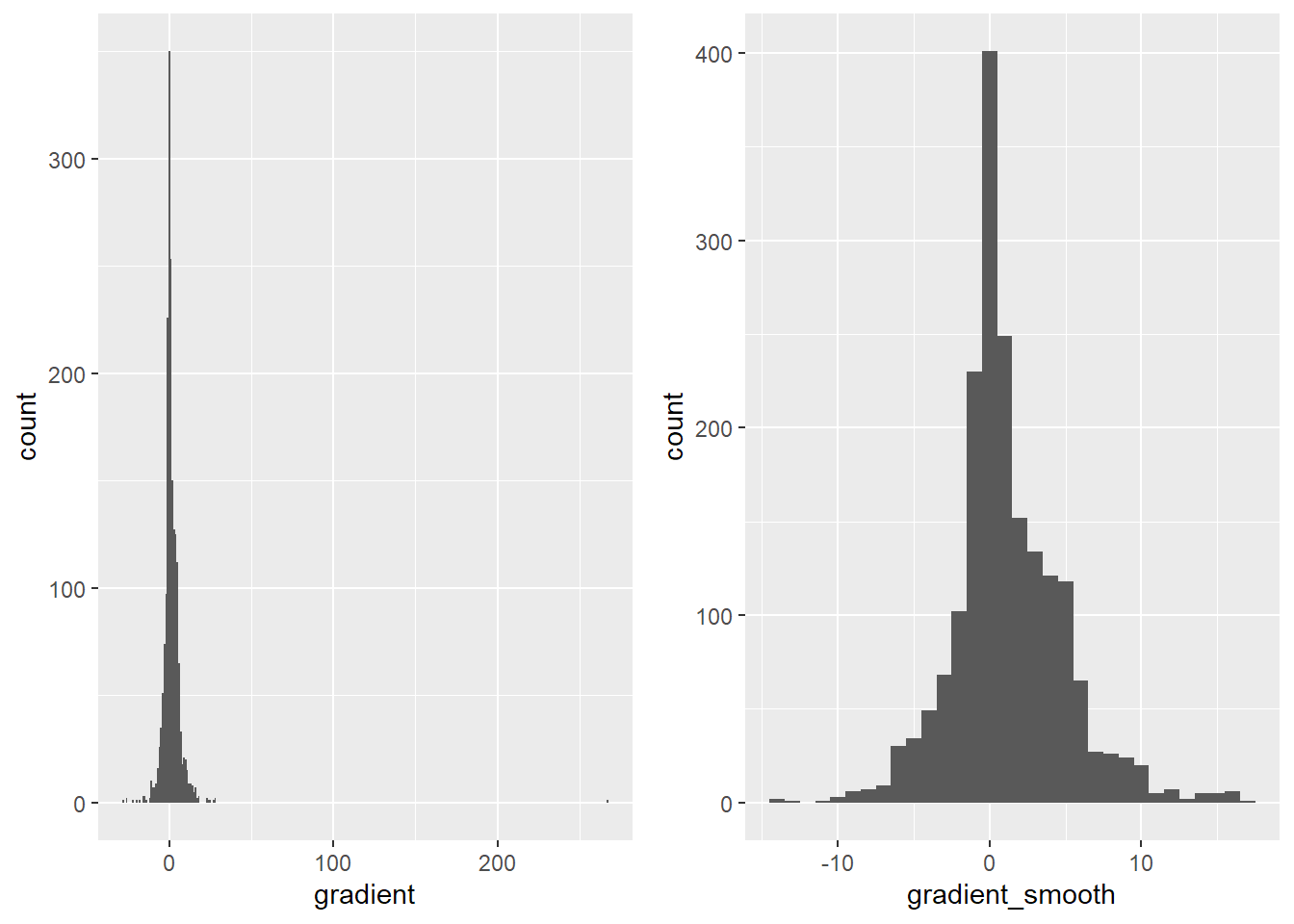
Code
tm_shape(bike_gradient) +
tm_dots("gradient_smooth")Segmentation
In a next step, the data was segmented based on a gradient threshold of 3% ((Parkin and Rotheram 2010), (Castro, Johansson, and Olstam 2022)). To create the segments, a function was used from GEO880. It creates an ID for each point, based on run length encoding from R. A Boolean column was created based on the threshold, one for whether the gradient is steep uphill and one for whether it is steep downhill. In this column, if a point that was steep was followed and preceded by non-steep points, it was also assigned non-steep. In essence, a moving window was run so that there are no segments that only consist of one point. The ID function then assigns an ID to all True values until there are False values, for which it assigns a new ID and so on. The result of the segmentation can be seen in Figure 9.
Code
bike_gradient <- bike_gradient |>
  mutate(
    steep_up = gradient_smooth > 3,
    steep_down = gradient_smooth < -3
  )

#removing single TRUE/FALSE values
# REVIEW AGAIN; JUST TO MAKE SURE IT IS CORRECT; CHECK
bike_gradient <- bike_gradient |>
  mutate(
    steep_up = ifelse(!steep_up, lag(steep_up) & lead(steep_up), steep_up), #if both are TRUE, make it also TRUE, otherwise take the initial value.
    steep_up = ifelse(steep_up, lag(steep_up) | lead(steep_up), steep_up), #if either (or both) are true, then the value stays true. If both are FALSE, it will also be FALSE, otherwise keep the TRUE value.
    steep_down = ifelse(!steep_down, lag(steep_down) & lead(steep_down), steep_down),
    steep_down = ifelse(steep_down, lag(steep_down) | lead(steep_down), steep_down)
  )

rle_id <- function(vec) {
    x <- rle(vec)$lengths # vector that gives the length of TRUE/FALSE values in a sequence (e.g. 2(TRUE) 3(FALSE) 1(TRUE))
    as.factor(rep(seq_along(x), times = x)) #assigns id along the data, repeating an ID as many times as defined in the lengths from the rle
}

bike_gradient <- bike_gradient |>
    mutate(segment_id_up = rle_id(steep_up),
           segment_id_down = rle_id(steep_down))

tm_shape(bike_gradient) +
tm_dots("segment_id_up") The data was put into a new data frame, by summarizing segments and grouping by uphill and downhill segment ID, which allows a unique distinction between flat, uphill and downhill parts. Then the speed difference between the average speed of a flat part before and a flat part directly after an uphill segment was calculated (Table 2). To test H1, a regression model was used which tests whether the average gradient of the uphill slope is a good predictor of the speed difference.
Code
avg_speeds <- bike_gradient |>
  group_by(segment_id_up, segment_id_down) |>
  summarise(
    seg_avg = mean(speed),
    uphill = ifelse(all(steep_up), TRUE, FALSE),
    flat = ifelse(all(!steep_up & !steep_down), TRUE, FALSE),
    downhill = ifelse(all(steep_down), TRUE, FALSE),
    avg_grad = mean(gradient_smooth)
  )

#couldn't figure out a working vectorized version.
#loops over rows, calculates a speed on uphill rows, that are followed and preceded by flat parts
#doesn't consider the first and last row (due to no preceding/following segments)
avg_speeds <- avg_speeds |>
  mutate(speed_diff = 0)

for(i in 2:(nrow(avg_speeds)-1)) {
  if (avg_speeds[i, ]$uphill & avg_speeds[i+1, ]$flat & avg_speeds[i-1, ]$flat){
    avg_speeds[i, ]$speed_diff <- avg_speeds[i-1, ]$seg_avg - avg_speeds[i+1, ]$seg_avg
  }
  else {
    avg_speeds[i, ]$speed_diff <- NA
  }
}

knitr::kable(head(avg_speeds, n =3))| segment_id_up | segment_id_down | seg_avg | uphill | flat | downhill | avg_grad | geometry | speed_diff |
|---|---|---|---|---|---|---|---|---|
| 1 | 1 | 17.687067 | NA | NA | NA | NA | POINT (2673909 1249682) | 0.000000 |
| 2 | 2 | 17.129494 | FALSE | TRUE | FALSE | 2.475004 | MULTIPOINT ((2673778 124968… | NA |
| 3 | 2 | 9.472181 | TRUE | FALSE | FALSE | 5.789082 | MULTIPOINT ((2673638 124971… | 2.522872 |
Results
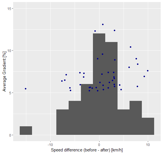
The results of the summary and the regression (as can be seen below and in Figure 10) do not indicate a relationship between speed difference and uphill gradient. With an R-squared value of 0.03 and a p-value of 0.24, there is no explanation of the variance in speed by the uphill gradient.
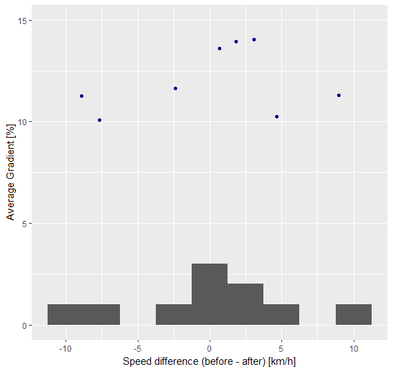
To check if the method is flawed or if the results are influenced by the choice of gradient for ‘steepness’, two more runs were made, one with a gradient threshold for steepness of 5% and with 10% (based roughly on (Winters et al. 2016) and (Duc et al. 2008)). The 5% run looks like it has the same issue like the 3% run, with a lot of points having negative speed differences, meaning that the cyclist got faster after a steep part (see Figure 11 (a)). It created a similar amount of steep segments that were used for the analysis (49 vs 44), which means that there are not many segments between 3 and 5%. It also had a very low R-squared value of 0.066. The p-value of 0.091 actually tends towards significance, but it is still not statistically conclusive. In the 10% run (Figure 11 (b)), the results looked similar to the other two, this time only 23 segments were created, due to the high steepness threshold. 8 of these segments were steeps followed and preceded by flats and therefore used in the linear regression. The R-squared value of 0.073 and p-value of 0.517 also mean that the gradient is not good in explaining the variance in speed difference around the steep parts.
H1 has to be rejected, as there is conclusive evidence that the speed difference can not be attributed to the slope gradient.
Code
reg <- lm(avg_speeds$speed_diff~avg_speeds$avg_grad)

#get intercept and slope value
coeff<-coefficients(reg)
intercept<-coeff[1]
slope<- coeff[2]

# library(xtable)
# knitr::kable(xtable(summary(reg)), format="markdown", align="c")
#https://github.com/mgimond/Stats-in-R/blob/gh-pages/regression.qmd

summary(reg)
Call:
lm(formula = avg_speeds$speed_diff ~ avg_speeds$avg_grad)

Residuals:
     Min       1Q   Median       3Q      Max
-12.6774  -3.3251   0.1111   2.7009  13.1989

Coefficients:
                    Estimate Std. Error t value Pr(>|t|)
(Intercept)          -0.5425     2.5585  -0.212    0.833
avg_speeds$avg_grad   0.5601     0.4668   1.200    0.236

Residual standard error: 5.384 on 47 degrees of freedom
  (117 observations deleted due to missingness)
Multiple R-squared:  0.02972,   Adjusted R-squared:  0.009078
F-statistic:  1.44 on 1 and 47 DF,  p-value: 0.2362
Code
avg_speeds |>
  ggplot()+
  geom_histogram(aes(speed_diff), binwidth = 2.5)+
  geom_point(aes(speed_diff, avg_grad), color = "darkblue")+
  xlab("Speed difference (before - after) [km/h]")+
  ylab("Average Gradient [%]")+
  ylim(0, 15)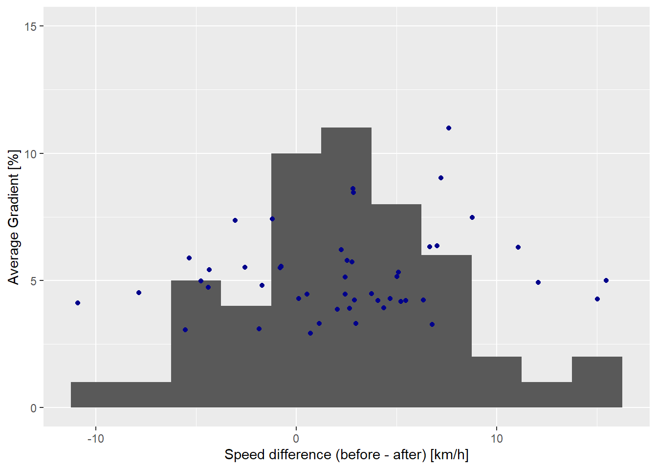
Limitations
This study is limited by the summary of segments. The initial idea was to treat every point individually and being able to see distinguished speed differences. By summarizing the segments into one average speed and slope, the calculation is faster and less complicated, but the results show that the method does not fit the study. The fact that there are a lot of flat segments following steep segments that increase in speed, probably means there is an issue in the methodology. Even if the methodology is fine (which could be the case, but the results are unintuitive), the analysis would be more geared towards the proposed research hypothesis if the speed increase/decrease would be measured for individual points of subsegments. H2 and H3 can not be tested with this approach either.
Another issue with how the experiment is at the moment is that a flat part can be after a steep part and at the same time in front of a steep part. This means that if the cyclist is tired after the first steep part this shows in the speed difference of the first steep part, but then another hill comes and the cyclist might recover only after the second one, which results in the second steep part having a speed increase afterwards. When looking at the scatterplots (Figure 10, Figure 11 (a), Figure 11 (b)) and the data frames, it seems possible that this happens fairly often. At least that is the most obvious explanation in my opinion.
There is also a limitation in data availability. With more data, there is a possibility that the trend would be stronger in either direction. As it stands the data does not have great statistical significance.
One last issue is, that the author had to fulfill their civic duties and went to the military in the last few weeks of the project, which hindered its development.
Discussion
Segmenting the data worked fairly well. The verification was done visually with Figure 9, where a point can be clicked to see the segment id. Some known points of steepness change were looked at (for 3% gradient threshold segmentation) and it looked very promising. Not a single steepness change was found that does not change the segment. There were very few segments that might have been split too much (e.g. 93-95), but over all there were not many issues. This over-segmentation could have had an influence on the result, but with enough data it should not be significant.
With multiple runs with varying steepness, there can be two conclusions. One is that the results are true and indicate that cyclists do not tend to slow down after a steep hill. The other is that the method is flawed and would have to be improved to draw a good conclusion from the results. Personally, I tend towards the second one. One key issue with the 10% methodology is that ‘flat’ segments would be including up to 10% gradient, which is certainly not true. There would have to be a separate function to determine flatness for the 10% case, which is not easily implemented with the function used here.
As there is not much literature on the topic, I will discuss here what I think has to be done to further this research. With more time I could have implemented more of it, but I had to go to the military and did not have much free time. As the main issues seem to be the averaging of speeds and slope gradients, and flat segments being potentially both before and after steep segments, the best way to counteract that would be to use the points individually. Maybe there is a way to calculate the speed difference for each point after a steep segment to an average before the segment and if the speed difference turns positive after a few points, the recovery has set in. This could then be used as a point to segment the flat part into ‘after steep’ and ‘before steep’ parts. There could also be a statistic of how long it takes the cyclist to recover and whether there is a fatigue and training effect, which could answer H2 and H3.
Before this project was started, it was clear that segmenting in a meaningful way will be the biggest challenge and it did remain exactly that.
When trying to fit this movement pattern, if it can be called that, into the taxonomy of movement patterns as proposed by Dodge, Weibel, and Lautenschütz (2008), is a bit tricky. It surely belongs to the generic patterns and is likely an isolated object compound pattern as only a single cyclist is researched even if they rarely ever belong to a flock. It could also be called a trend/fluctuation pattern as the change in speed fluctuates after a hill, but was hypothesised to follow a trend. It probably is both and cannot be just attributed to one simple category.
Conclusion
This project tried to lay a framework for analysing the speed differences of a cyclist when going over steep hills. It successfully aggregated data from a GPS tracking platform with height data from a high resolution DEM, and calculated speed, gradient and excluded stops. It failed in conclusively showing how to define a steep hill, with the most promising statistical results coming from a 5% slope gradient threshold. A plan was formulated how to improve this approach in any future research, but it could not be implemented in time.
Acknowledgement
Thank you to Nils Ratnaweera. Without him the memory of my laptop would be burnt out and the DEM would not have loaded.