library(sf)
library(tmap)

# Get a sample road dataset
HighWays <- read_sf(system.file("sqlite/test3.sqlite",package="sf"), "HighWays")[6, ]

# since we want to find the closest location on the road over ALL roads
# we need to create a union of the roads first.
HighWays <- st_union(HighWays)

# Let's simulate 1000 GPS locations within 3km of the highway
gps_locations <- HighWays |> st_buffer(3000) |> st_sample(100)

# Now we can get the nearset point for each GPS location
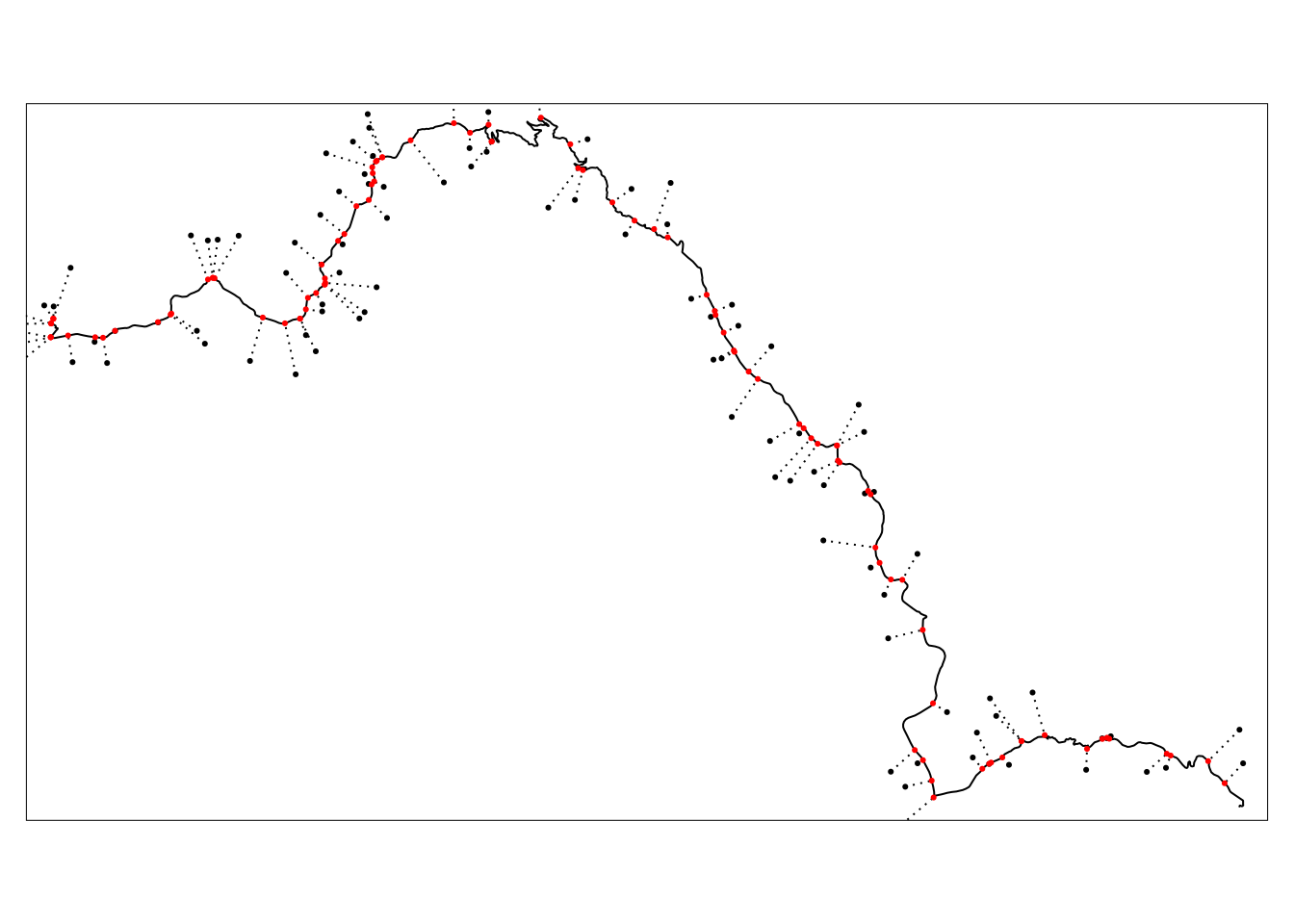
nearest <- st_nearest_points(gps_locations, HighWays)

# The output is a line for each point (see plot below)
# Now we need convert the output from LINE to POINT.
# This doubles the number of features
near_p <- st_cast(nearest, "POINT")

# now we subset the points. Uneven numbers are the original
# points, even numbers are the new, mapmatched points.
near_from <- near_p[c(TRUE, FALSE)]
near_to <- near_p[c(FALSE,TRUE)]Appendix
Data-import: base-r vs readr
Our reasons for preferring readr over base-R import functions:
base(since R 4.0.0, this is not the case anymore)Rimports strings as factors by defaultreadris generally faster (which only matters if you have a large dataset)readrmakes safer assumptions about your data (e.g. the default timezone for datetime columns is UTC)data.framescreated byreadrare prettier when printed to the console and contain more information using less characters
HOWEVER: Using external libraries (such as readr) creates additional dependencies which has it’s own downsides (which is one of the reasons we don’t do library("tidyverse")).
Comitting files with git
Note 24.1: Committing files with git
- Save your (R/RMarkdown/Quarto) file
- Switch to the “Git”-Tab in the pane in the top right corner
- Click “commit” to open the “Commit Window”
- Click in the checkbox next to the file(s) you want to commit
- Add a commit message to explain what you are committing (e.g. “
initial commit”) - Click on “commit” to commit your changes
Mapmatching GPS points to the road network
tm_shape(HighWays) + tm_lines() +
  tm_shape(nearest) + tm_lines(lty = 3) +
  tm_shape(near_from) + tm_dots() +
  tm_shape(near_to) + tm_dots(col = "red")
Exporting location data from Google
A simple way to download your location data from Google is described in the following steps:
- Go to takeout.google.com
- Deselect all “Products” and select only the following product: Location History (Timeline)
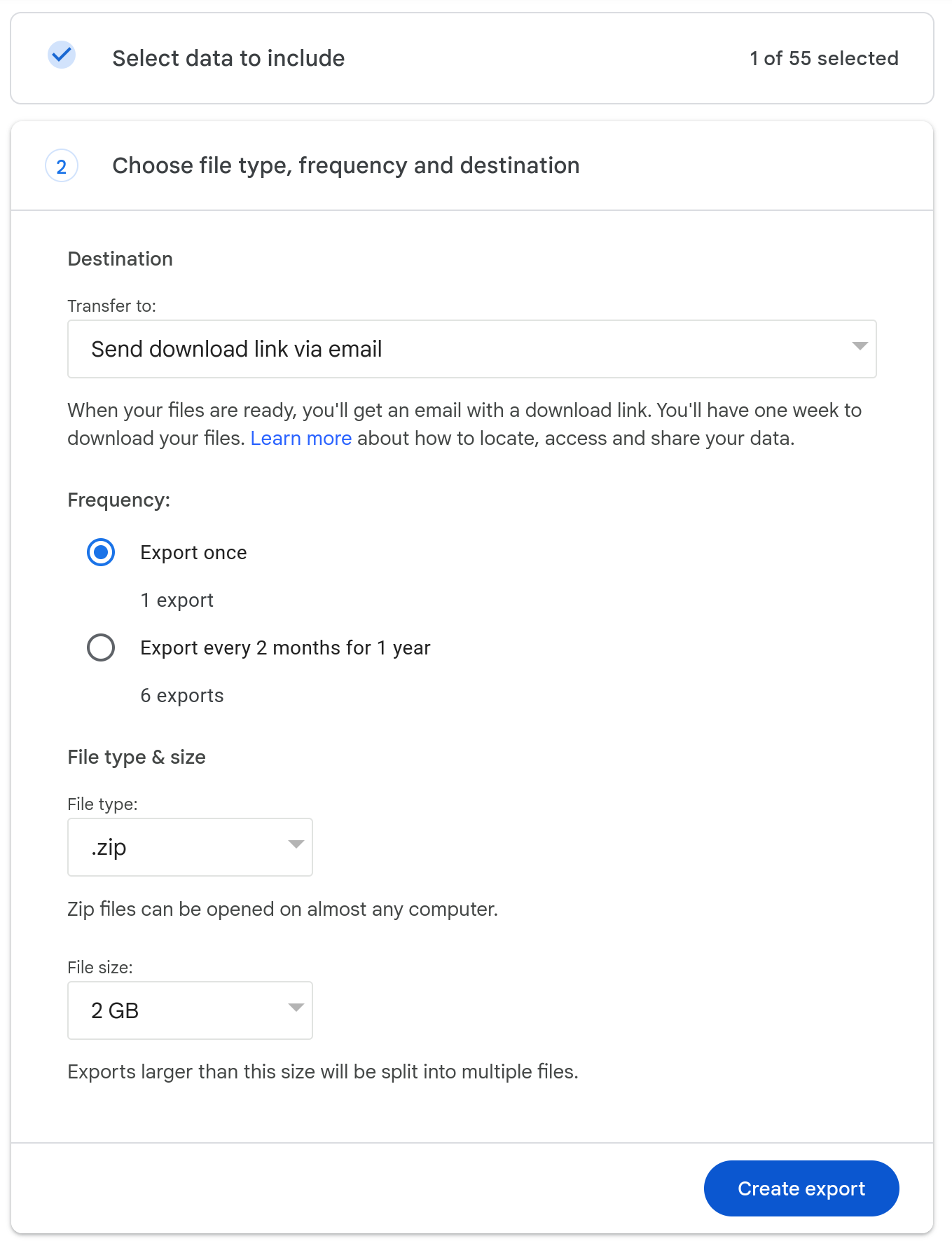
- Click Next and Create Export to get an Export of your data (see Figure 24.1)
- Download and extract the data in your R-Project folder
- Follow the script below (adjust the path!)
library(sf)
library(jsonlite)
library(dplyr)
records_json <- jsonlite::read_json("takeout-20240501T094208Z-001/Takeout/Location History (Timeline)/Records.json",simplifyVector = TRUE)

records <- records_json[[1]]

# inspired by the following SO-answer
# https://gis.stackexchange.com/a/319067/40929
records_sf <- records |>
  mutate(
    lat = latitudeE7/1e7,
    lon = longitudeE7/1e7
  ) |>
  st_as_sf(coords = c("lon", "lat"), crs = 4326)
