Tasks and inputs

Up to now, we have used a variety of different functions designed by other developers. Sometimes we need to execute an operation multiple times, and most often it is reasonable to write a function to do so. Whenever you have copied and pasted a block of code more than twice, you should consider writing a function (Wickham and Grolemund 2017).

The first step in writing a function, is picking a name and assigning <- function(){} to it.

testfun <- function() {}

To run the function, we have to call the assigned name with the brackets. The function testfun gives no output, which is why we get NULL back.

testfun()

NULL

class(testfun)

[1] "function"

To make the function actually do something, we need to specify what should be done within the curly brackets {}. The following function always prints the same statement and accepts no input values:

testfun <- function() {
    print("this function does nothing")
}

testfun()

[1] "this function does nothing"

If we want the function to accept some input values, we have to define them within the round brackets. For example, I specify a variable named sometext and can call this variable within the execution.

testfun <- function(sometext) {
    print(sometext)
}

testfun(sometext = "this function does slightly more, but still not much")

[1] "this function does slightly more, but still not much"

Note

testfun <- function(sometext) {
    print(sometext)
}

Note that since R Version 4.1, the above syntax can also be written as follows:

testfun <- \(sometext){
    print(sometext)
}

or even more compact:

testfun <- \(sometext) print(sometext)

Let’s take a more practical example. Say we want a function that calculates our age if provided with the date of our birthday. We can use Sys.time() to provide today’s date and difftime() to calculate the time difference between today and our birthday.

my_age <- function(birthday, output_unit) {
    difftime(Sys.time(), birthday, units = output_unit)
}

my_age(birthday = "1997-04-23", output_unit = "days")

Time difference of 9907.618 days

As we already know from using other functions, if we declare our variables in the order that we initially listed them, we do not need to specify the parameters (no need of birthday = and output_unit =).

my_age("1997-04-23", "days")

Time difference of 9907.618 days

If we want any of our parameters to have default value, we can assign an initial value to the parameter when declaring the variables within the round brackets.

my_age <- function(birthday, output_unit = "days") {
    difftime(Sys.time(), birthday, units = output_unit)
}

# if not stated otherwise, our function uses the unit "days"
my_age("1997-04-23")

Time difference of 9907.618 days

# We can still overwrite units
my_age("1997-04-23", "hours")

Time difference of 237782.8 hours

All you need to do now is run execute the function deceleration (myage <- function... etc.) at the beginning of your script, and you can use the function for your entire R session.

Important

Always try to make your function self sufficient: Only use objects within your function that are either passed as function arguments or created within the funtion. See more on this topic here, in the online version of the book by Rodrigues (2023).

Task 1: Write your own functions

Create the following two functions:

1. A function which calculates a persons BMI based on their height and weight (\(\text{BMI} = \frac{\text{Weight (kg)}}{\text{Height (m)}^2}\))
2. A function which converts degrees Celcius to Farenheight (\(\text{Farenheight} = \text{Celcius} \times \frac{9}{5} + 32\))
3. A function which calculates the (Euclidean) distance between two sets of coordinates (\(x_1\), \(y_1\) and \(x_2\), \(y_2\)) based on the formula below:

\[\text{Euclidean distance} = \sqrt{(x_2 - x_1)^2+(y_2 - y_1)^2}\]

Task 2: Prepare Analysis

In the next tasks we will look for “meet” patterns in our wild boar data. To simplify this, we will only use a subset of our wild boar data: The individuals Rosa and Sabi for the timespan 01.04.2015 - 15.04.2015. You can download the dataset here wildschwein_BE_2056.csv. Import the csv as a data.frame and filter it with the aforementioned criteria. You do not need to convert the data.frame to an sf object.

Task 3: Create Join Key

Have a look at your dataset. You will notice that samples are taken at every full hour, quarter past, half past and quarter to. The sampling time is usually off by a couple of seconds.

To compare Rosa and Sabi’s locations, we first need to match the two animals temporally. For that we can use a join, but need identical time stamps to serve as a join key. We therefore need to slightly adjust our time stamps to a common, concurrent interval.

The task is therfore to round the minutes of DatetimeUTC to a multiple of 15 (00, 15, 30,45) and store the values in a new column¹. You can use the lubridate function round_date() for this. See the examples here to see how this goes.

Your new dataset should look something like this (note the additional column):

# A tibble: 6 × 7
# Groups:   TierID [1]
  TierID TierName CollarID DatetimeUTC              E      N DatetimeRound      
  <chr>  <chr>       <dbl> <dttm>               <dbl>  <dbl> <dttm>             
1 002A   Sabi        12275 2015-04-01 00:00:11 2.57e6 1.21e6 2015-04-01 00:00:00
2 002A   Sabi        12275 2015-04-01 00:15:22 2.57e6 1.21e6 2015-04-01 00:15:00
3 002A   Sabi        12275 2015-04-01 00:30:11 2.57e6 1.21e6 2015-04-01 00:30:00
4 002A   Sabi        12275 2015-04-01 00:45:16 2.57e6 1.21e6 2015-04-01 00:45:00
5 002A   Sabi        12275 2015-04-01 01:00:44 2.57e6 1.21e6 2015-04-01 01:00:00
6 002A   Sabi        12275 2015-04-01 01:15:17 2.57e6 1.21e6 2015-04-01 01:15:00

Task 4: Measuring distance at concurrent locations

To measure the distance between concurrent locations, we need to follow the following steps.

1. Split the wildschwein_filter object into one data.frame per animal
2. Join* these datasets by the new Datetime column created in the last task. The joined observations are temporally close.
3. In the joined dataset, calculate Euclidean distances between concurrent observations and store the values in a new column
4. Use a reasonable threshold on distance to determine if the animals are also spatially close enough to constitute a meet (we use 100 meters). Store this Boolean information (TRUE/FALSE) in a new column

* We recommend using one dplyrs join methods (inner_join(), left_join(), right_join() or full_join()), which one is appropriate? Tip: specify suffix to prevent column names ending in .x or .y.

Task 5: Visualize data

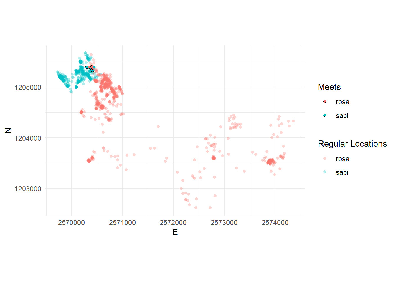
Now, visualize the meets spatially in a way that you think reasonable. For example in the plot as shows below. To produce this plot we:

• Used the individual dataframes from rosa and sabi (from the previous task)
• Used the joined dataset (also from the previous task), filtered to only the meets
• Manually changed the x and y axis limits

Task 6 (optional): Visualize data as timecube with plotly

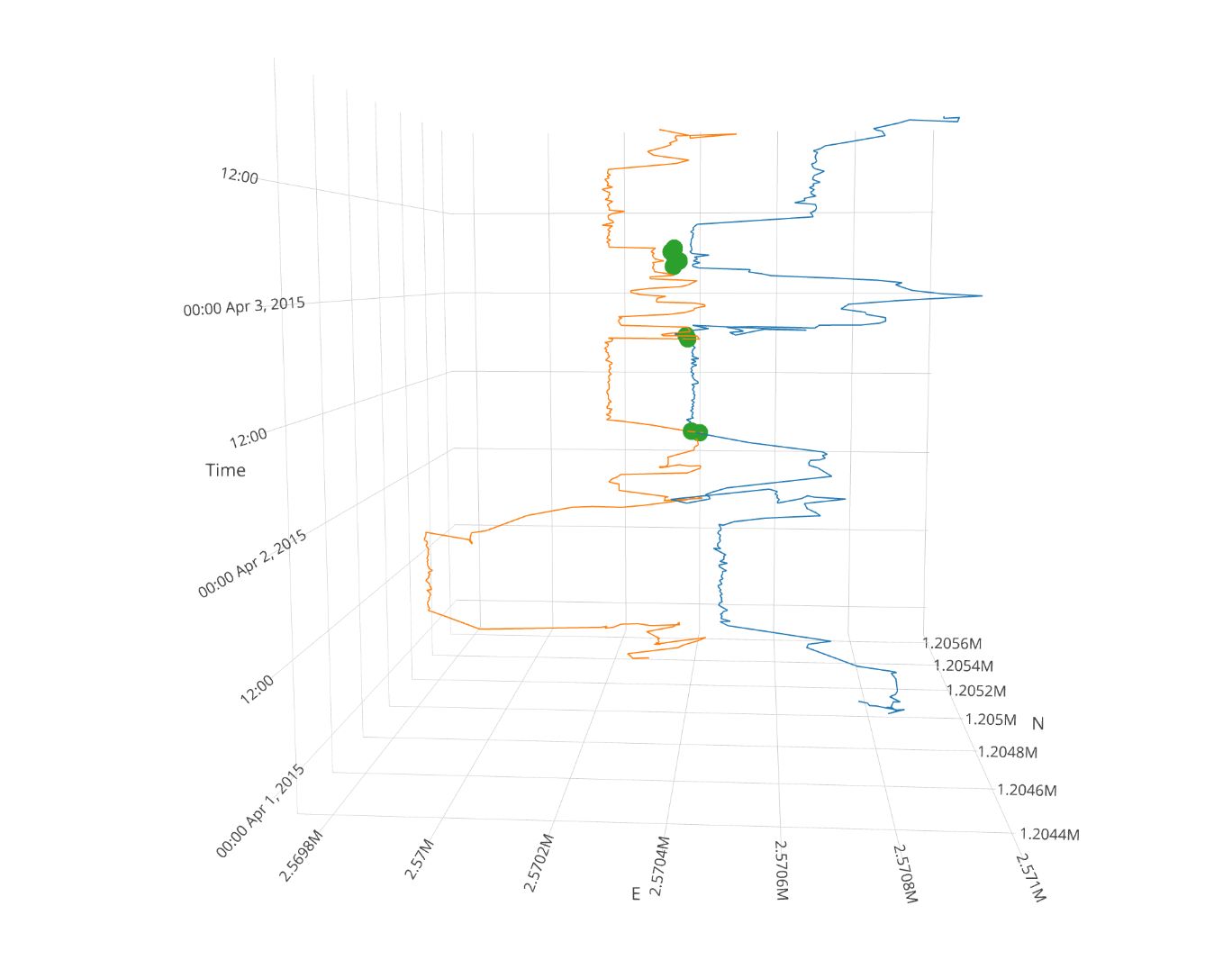
Finally, you can nicely visualize the meeting patterns and trajectories in a Space-Time-Cube (Hägerstraand 1970) with the package plotly. There are some nice ressources available online.

Submission

To submit your exercise, provide us with the URL of your Github repo as described in the preperation.

You can give other GitHub users write access to your repository throught the repository settings. You will be needing this for your semester project. To practice this, add Dominic (@DLND8) and Nils (@ratnanil) to your GitHub repo:

1. Go to your GitHub repository on GitHub.com
2. Go to the repository settings by clicking on the Settings tab
3. In the left panel, click on Collaborators and teams and then Add people
4. Add the mentioned Persons via their GitHub Usernames, give them Write privilages.

Hägerstraand, Torsten. 1970. “What about People in Regional Science?” Papers in Regional Science 24 (1): 7–24.

Rodrigues, Bruno. 2023. Building Reproducible Analytical Pipelines with r. leanpub.

Wickham, Hadley, and Garrett Grolemund. 2017. R for Data Science: Import, Tidy, Transform, Visualize, and Model Data. 1st ed. O’Reilly Media, Inc.

---

1. Please note: We are manipulating our time stamps without adjusting the x,y-coordinates. This is fine for our simple example, but we would advice against this in a more serious research endeavour, e.g. in your semester projects. One simple approach would be to linearly interpolate the positions to the new timestamps. If you choose Option A the wild boar projects as your semester projects, you should aim for a linear interpolation. Get in touch if you need help with this.